ROC curve-what you always wanted to know but were afraid to ask…

This post is inspired, as many of them, by the student’s question. It appears that many of us use ROC curves in the analysis not really knowing what these curves are for and how they are created.

The classification models have become a very popular tool and are part of many implemented widely available black-box solutions, often as a part of machine learning tools. On one hand, this easy availability of ready-to-use tools is very tempting and encourages people to try them. On the other, since it is given, nobody seeks additional knowledge about the method. Very often one does not see the implemented code of such classification models. Therefore, it is not clear what hides behind that black box.

Let’s take an example from medicine. Let us assume that we have a binary 0-1 response, denoting if a patient is sick (1) or healthy (0). In addition, we have some data about the patients that we think or know might be the potential predictors for the probability of being sick or healthy, such as Age, BMI, Gender, or Smoking. The model that connects our binary predictor with the set linear combination of the predictors is called the logistic regression model. It is the generalization of well known linear normal regression model but this time our response is binary, not continuous and we need to connect this binary response with the linear part of the model. That happens via the so-called link function, which is a logit function for the logistic regression model. In R the code to fit a logistic regression model is as follows:

my_model<-glm(binary_response~ age + smoke + bmi + gender,family=binomial, data=my_data))
summary(my_model)

The model above might be a final model after applying some piecewise building procedure to get the final set of significant predictors. Or we might want to test those predictors on our data knowing from literature they have been found to be significant in other studies.

Note that we build models for two reasons:

1. For inference, to drive the conclusions. Then we really should eliminate those not significant predictior using for example some backward elimination procedure.
2. For prediction purpose. Then the model can be overrfitted. We do not care so much about what is in as long as it has good prediction ability.

Let us focus on this second purpose because that is where the ROC curve comes in handy. But first things first. After fitting the model we want to see how good the prediction from that model is. Ideally, we should build/train our model on the so-called training set and then test it on the other testing set. It can be the same data but we just use a part of it as a training part and another part as the testing part. The question that arises is in which proportion we should do it. It is not trivial and it is a subject of so-called cross-validation methods. Ideally, we should examine different splits and repeat this procedure by randomly sampling from our data. For now, let us assume that we had our pilot data which was used to build a model, and that now we have new data for which we want to check the performance of our model.

First we create predictions of our response from the fitted logistic model.

predicted<-predict(my_model,type=c("response"))

It is important to realize that it will be a probability that is predicted, not a binary response. Let’s say for patient X the prediction was 0.7. Is that mean that he/she is sick? Well, if we assume that everyone with a probability >0.5 is sick then yes, he/she is sick according to our model. The choice of threshold 0.5 is here crucial. After we choose for example 0.5 we can examine the model performance.

predicted.threshold <- as.integer(predicted > my_threshold)

If we choose my_treshold to be 0.5 then precited.treshold response will be binary. It will be 1 for those probabilties >0.5 and 0 otherwise. We then can look at the confusion matrix.

table(my_data$binary_response,predicted.threshold)

predicted.threshold
    
      0   1
  0  25 304
  1  13 258

From that confusion matrix, we can see how many false positive (FP) observations we have, which are those predicted by the model as sick (1) but they are healthy. In addition, we will have false negative (FN) observations, which are those predicted as healthy, but in fact, are sick. The rest of the observations will be true positives (TP), predicted correctly as sick and true negatives (TN), predicted correctly as healthy.

The common measure to assess the model performance is sensitivity=TP/P, which is the proportion of all sick patients (P) detected as sick . A second measure is so-called specificity=TN/N, which is the proportion of all healthy patients detected as healthy.

Now, nobody tells us that our threshold must be 0.5. Why not 0.6? If we change the threshold, the predictions will change, the confusion matrix will change and the sensitivity and specificity will change.

How to choose this threshold to maximize specificity and sensitivity? The idea is to have them both high. But once sensitivity goes up the specificity goes down and vice versa. It is a trade-off between these two.

So do we need to run the code for all those possible thresholds? No, the ROC curve will do that for us.

library(pROC)

myROC<- roc(my_data$binary_response ~ predicted)

plot(myROC)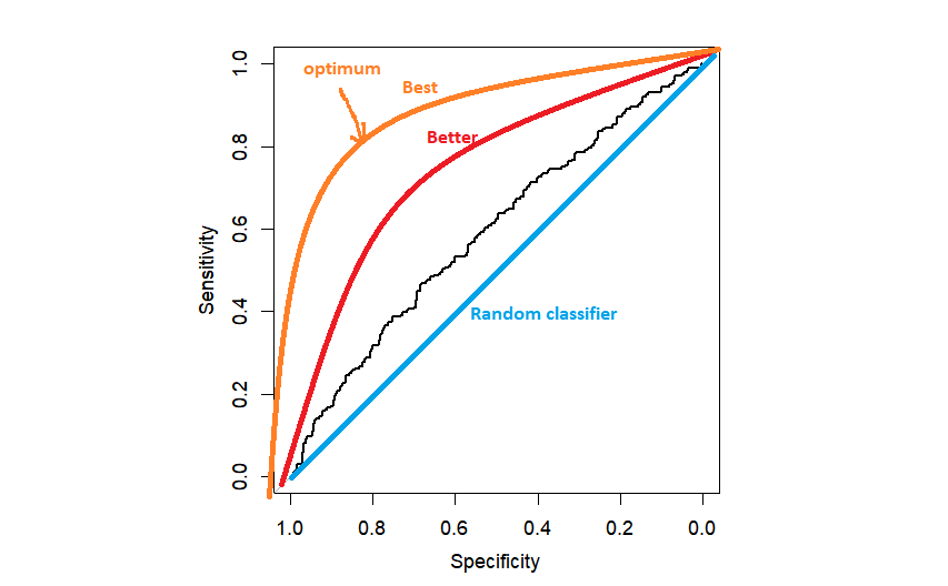

In practice, we might get something like the black ROC curve, just a bit better than a random classifier. The closer to the left upper corner the ROC is, the better because we are closer to the maximum specificity=1 and maximum sensitivity=1.

The next question is how to choose the threshold. The most popular method is choosing the threshold that maximizes the distance to the left upper corner. It can be done automatically by R, but it is good to program it once by yourself.

topleft<-(1-myROC$sensitivities)^2+(1-myROC$specificities)^2
topleft.threshold<-which(topleft==min(topleft))
text(x=myROC$specificities[topleft.threshold], y=myROC$sensitivities[topleft.threshold],"(0.50,0.58)",col=2)

Once we found that optimal point we can put it on the graph using the text function. At that point, one usually stops, reporting finally AUC (area under the curve) as the total predictive ability of the model. But we should not stop here. We want to find out which threshold (the cutoff point) corresponds to the optimal sensitivity and specificity point.

#for a given sensitivity and specificity
idx.which<-which((myROC$specificities==0.50)&(myROC$sensitivities==0.58))

#now we take threshold
myROC$thresholds[idx.which]

predict.treshold <- as.integer(predicted > myROC$thresholds[idx.which])
#confusion matrix
table(my_data$binary_response,predict.threshold)

Now we have found the optimal threshold myROC$thresholds[idx.which] and we can use it to cut our predicted probabilities.

As I mentioned before, the area under the ROC curve is commonly used as the criterion to summarize the overall prediction ability of our model. It is good to realize that it is the ability across all possible thresholds. The closer to 1, the better. AUC for the random classifier is equal to 0.5, which corresponds to the area under the diagonal line on the plot above.

The classification models are of course much larger family than just the logistic regression models. It is a broad topic of the research. It is good to know that there are other methods, apart from “top-left” corner to choose the optimum criteria such as Jouden’s. This criterion treats sensitivity and specificty equally important. But this is not always the case. One needs to look at the particular data in hand because your setting might be completely different than that in someone’s else tutorial. Coming back to the medical example. If your disease is the cancer you are more worried about the false negative observations than about the false positives. Those false positives will be further diagnosed but missing some cancer patients might cause their death. In that setting you will rather maximize sensitivity for the cost of the specificity. On the other hand, if your disease is an HIV you are probably equally concerned about both, false negative and false positive patients.

Good luck with your models!