Mixed ANOVA in R

Suppose we have a data of the form:

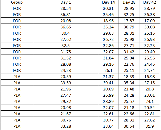
And we would like to know if there was any group, time, or group*time interaction effect.

First we read the data and tranform it the into a long format:

library(openxlsx)

library(lme4)
library(afex) #for p-values

library(ggplot2)
library(gtsummary)#for nice tables

#read the data (put the path to your file here)
data.rep<-read.xlsx ("C:/Users/mmura/OneDrive/Dokumenty/FB/data.xlsx")

head(data.rep)
dim(data.rep)

#make a data in a long format, adding some ID for individuals 

data.long<-as.data.frame(cbind(ID=rep(seq(1:20),4),time=rep(c(1,14,28,42),each=20),
          resp=c(data.rep$Day.1,data.rep$Day.14,data.rep$Day.28,data.rep$Day.42),
          group=rep(data.rep$Group,4)))
head(data.long)

data.long$time<-as.numeric(data.long$time)
data.long$resp<-as.numeric(data.long$resp)

At the same time, we add some ID variable for individuals. This could be plates/measures or whatever was measured under the changing conditions.

As the next step, we do some visualization:

#make some visualization

#individual profiles 
ggplot(data.long, aes(x=time, y=resp,color=ID)) + geom_smooth()+geom_point()+
  ylab("Your response")+xlab("Time (days)")

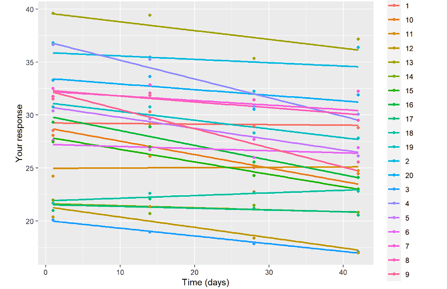
#now the linear by ID
ggplot(data.long, aes(x=time, y=resp,color=ID)) + geom_smooth(method = "lm",se=FALSE)+geom_point()+
  ylab("Your response")+xlab("Time (days)")

#from that we conclude about including random slopes as well

#smoothed by group 
ggplot(data.long, aes(x=time, y=resp,color=group)) + geom_smooth()+geom_point()+
  ylab("Your response")+xlab("Time (days)")

#now the linear by group
ggplot(data.long, aes(x=time, y=resp,color=group)) + geom_smooth(method = "lm",se=FALSE)+geom_point()+
  ylab("Your response")+xlab("Time")

We only show the linear plots below:

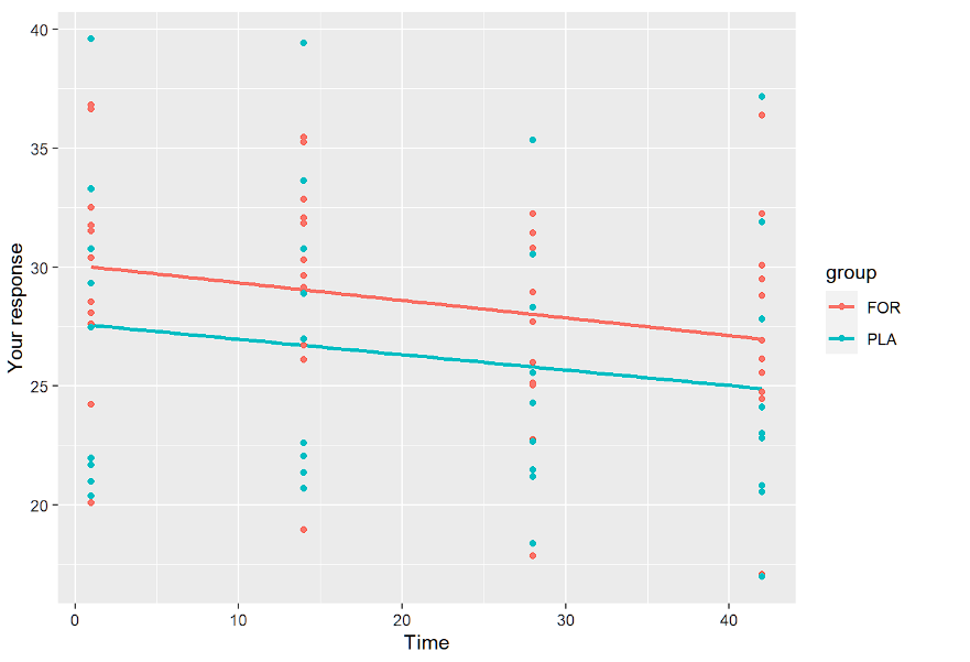
The purpose of those visualizations is to see if we need random intercept and slope and if the linear model seems to be the right one in the first place. Also, by inspecting by-group profiles we see what to expect. The profiles are parallel, so the group*time effect is not going to be significant.

Then we fit the initial model:

#fitting a model
m.initial<-lmer(resp~time*group+(1+time|ID),data=data.long)
summary(m.initial)
tbl_regression(m.final)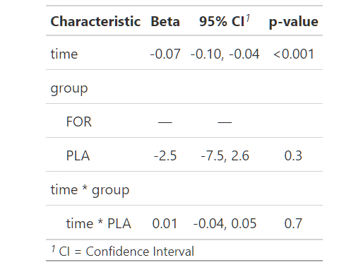

Since the interaction effect is not significant we remove it from the model:

#Since group*time is not significant we exclude it

m.2<-lmer(resp~time+group+(1+time|ID),data=data.long)
summary(m.2)

The main group effect is also not significant. Therefore, in the final model there will be only the fixed time effect:

m.final<-lmer(resp~time+(1+time|ID),data=data.long)
summary(m.final)


tbl_regression(m.final)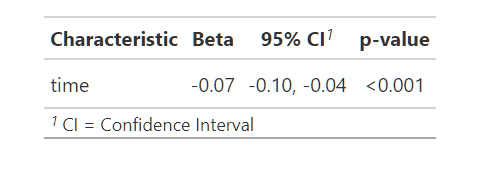

Therefore, the final conclusion is the following:

The negative trend effect is significant in the final mixed model. On average with every single day, the response decreases by 0.07 units.

The final RMD file is here.

And the data is here.