Pairwise comparisons

Post-hoc pairwise comparisons are very common part of the data scientist daily routine. Whenever we do ANOVA or non-parametric testing with more than two groups that is inevitable.

At some point you might want to have a nice visualizations of what is significant and what is not. Possibly with p-values written on the plot. Then you can think of some own-written function that does the job. Or you might find an ggpubr package as the easy solution. And here comes the trap. The usual code given as an example does not produce p-values adjusted for multiple comparisons! Let’s say you have some y response and 4 groups A, B, C , D and you would like to compare y in in other groups versus y in A reference group. Then you end up with the code like this:

library(tidyverse)
library(rstatix)   
library(ggpubr)
library(ggplot2)

my_comparisons <- list( c("A", "B"), c("A", "C"), c("A", "D"))

ggboxplot(data, x = "grouping.variable", y = "your.response",
          palette = "jco",fill="grouping.variable",order=c("A","B","C","D"),
          legend="right")+
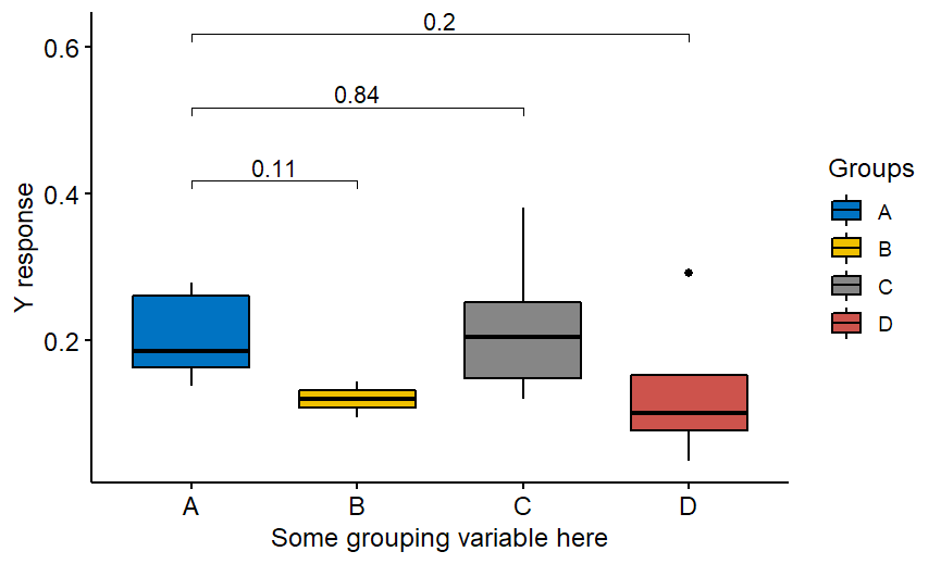
  stat_compare_means(comparisons = my_comparisons, label.y = c(0.4, 0.5, 0.6),method="wilcox.test",p.adjust.method = "bonferroni")+
  labs(y= "Y response",x= "Some grouping variable here",fill="Groups")

And the graph which does NOT have adjusted p-values!

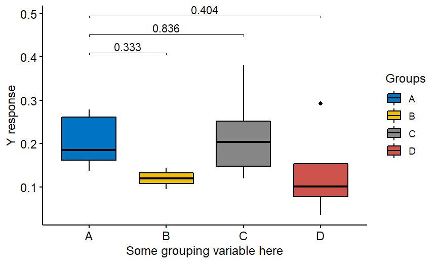
The correct code is the following:

stat.test <- data%>% 
  wilcox_test(your.response ~ grouping.variable,ref.group = "A") %>%
  adjust_pvalue() %>%
  add_significance("p.adj")
stat.test

stat.test <- stat.test %>% add_y_position()

ggboxplot(data, x = "grouping.variable", y = "your.response",
          palette = "jco",fill="grouping.variable",order=c("A","B","C","D"),
          legend="right")+stat_pvalue_manual(stat.test, label = "p.adj",tip.length = 0.01)+
  labs(y= "Y response",x= "Some grouping variable here",fill="Groups")

Of course above is an example with Wilcoxon nonparametric test but the package offers also t-test. If you would like to compare “everything with everything”, not only with the group A then just remove ref.group = “A” from the code:

stat.test <- data%>% 
  wilcox_test(your.response ~ grouping.variable) %>%
  adjust_pvalue() %>%
  add_significance("p.adj")
stat.test

stat.test <- stat.test %>% add_y_position()

ggboxplot(data, x = "grouping.variable", y = "your.response",
          palette = "jco",fill="grouping.variable",order=c("A","B","C","D"),
          legend="right")+stat_pvalue_manual(stat.test, label = "p.adj",tip.length = 0.01)+
  labs(y= "Y response",x= "Some grouping variable here",fill="Groups")

And you get:

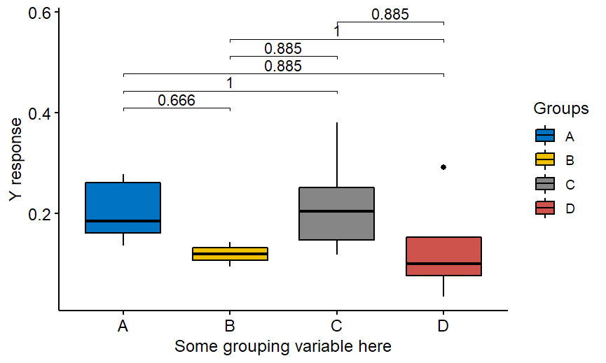
Note that the method of adjustment above is not Bonferroni anymore. It is Holm, a default method implemented in R. Have FUN!