百分比分离

假设您想让样本量达到某些百分位数，但又不想超标。代码如下

quantile.CI <- function(n, q, alpha=0.1) {
  #
  # Search over a small range of upper and lower order statistics for the 
  # closest coverage to 1-alpha (but not less than it, if possible).
  #
  u <- qbinom(1-alpha/2, n, q) + (-2:2) + 1
  l <- qbinom(alpha/2, n, q) + (-2:2)
  u[u > n] <- Inf
  l[l < 0] <- -Inf
  coverage <- outer(l, u, function(a,b) pbinom(b-1,n,q) - pbinom(a-1,n,q))
  if (max(coverage) < 1-alpha) i <- which(coverage==max(coverage)) else
    i <- which(coverage == min(coverage[coverage >= 1-alpha]))
  i <- i[1]
  #
  # Return the order statistics and the actual coverage.
  #
  u <- rep(u, each=5)[i]
  l <- rep(l, 5)[i]
  return(list(Interval=c(l,u), Coverage=coverage[i]))
}


###bootstrap alternative method############

quantile.CI.via.bootstrap <- function(x, p, alpha = 0.1) {
  ## Purpose:
  ##   Calculate a two-sided confidence interval with confidence level of (1 - alpha) for
  ##   a quantile, based on the (computing intensive) bootstrap resampling method. 
  ##
  ## Arguments:
  ##   - x: a vector of values, representing a data sample. 
  ##   - p: probability cutpoint for the quantile (between 0 and 1).
  ##   - alpha: type I error level (default to 0.1 so a 90% CI is calculated)
  ##
  ## Return:
  ##   - CI: the lower and upper limits of the two-sided CI. 
  
  q <- quantile(x, probs = p)         
  message("Quantile Point Estimate = ", q, " (Probability Cutpoint = ", p, ")\n")
  
  ## Bootstrap resampling with 2000 replications
  library(boot)
  set.seed(1)
  b <- boot(x, function(x, i) quantile(x[i], probs = p), R = 2000)
  
  boot.ci(b, conf = 1 - alpha, type = c("norm", "basic", "perc", "bca"))
  
}

第一种方法实现了 Hahn & Meeker 1991 年的方法，第二种方法只是一种非参数自举法。

n.s<-seq(50,200,5)

q.90<-0.90 #less strict
q.99<-0.99
results.90<-matrix(NA,2,length(n.s))
results.99<-matrix(NA,2,length(n.s))

for (i in 1:length(n.s)){
  
  lu.90 <- quantile.CI(n.s[i], q.90)$Interval
  results.90[1,i]<-lu.90[1]
  results.90[2,i]<-lu.90[2]
  
  lu.99 <- quantile.CI(n.s[i], q.99)$Interval
  results.99[1,i]<-lu.99[1]
  results.99[2,i]<-lu.99[2]
}


plot(results.90[2,],ylab="Estimated CI limit order",xlab="n",type="l",col="blue",axes=FALSE,pch=19)
轴（2）
axis(1, at=seq_along(results.90[1,]),labels=as.character(n.s), las=2)
box()
lines(results.99[1,],col="purple",type="l",pch=18)

abline(v = which(n.s==95), col="black", lwd=3, lty=2)
# 添加图例
legend(1, 175, legend=c("Lower Limit 99th", "Upper Limit 90th")、
       col=c("purple", "blue"), lty=1, cex=0.8)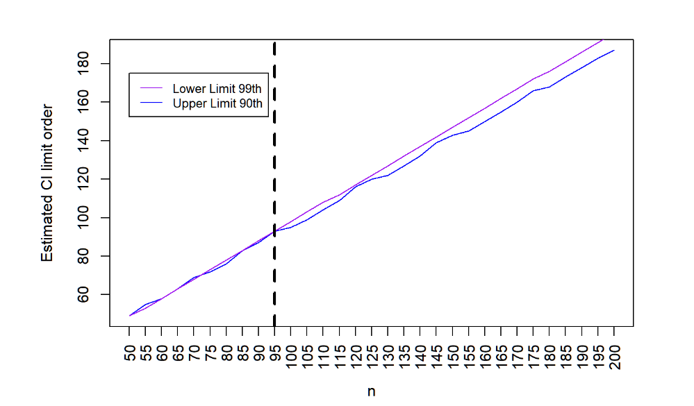

我们可以看到，根据引导法，样本 n=95 就足够了。

引导结果

n.s<-seq(50,200,5)
q.95<-0.90
q.99<-0.99
results.95<-matrix(NA,2,length(n.s))
results.99<-matrix(NA,2,length(n.s))


for (i in 1:length(n.s)){

  x <- rnorm(n.s[i], mean = which.mean.max, sd = which.sd.max) 1TP5这里有最大的 CV
  lu.95 <-quantile.CI.via.bootstrap(x, 0.90, 0.1)$bca
  results.95[1,i]<-lu.95[4]
  results.95[2,i]<-lu.95[5]
  
  lu.99 <- quantile.CI.via.bootstrap(x, 0.99, 0.1)$bca
  results.99[1,i]<-lu.99[4]
  results.99[2,i]<-lu.99[5]
}



plot(results.95[2,],ylab="Estimated CI limit",xlab="n",type="l",col="blue",axes=FALSE,pch=19,ylim=c(300,400))
轴（2）
axis(1, at=seq_along(results.95[1,]),labels=as.character(n.s), las=2)
box()
lines(results.99[1,],col="purple",type="l",pch=18)

abline(v = which(n.s==100), col="black", lwd=3, lty=2)
# 添加图例
legend(1,5 , legend=c("Lower Limit 99th", "Upper Limit 90th")、
       col=c("purple", "blue"), lty=1, cex=0.8)

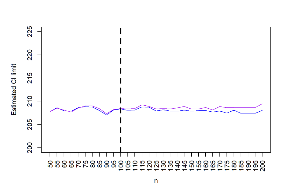
根据 boostrap 的结果，100 个样本就足够了。注意：这里使用的是自举样本中 BCA 类型的估计值，它是稳健型版本。

并不是说这两种方法都是无分布、非参数的！

您也可以将它们用于其他百分位数。玩得开心