

我们都知道常见的 OLS 线性回归模型。在这类模型中,我们假定 Y 与某个连续的预测因子 X 呈线性关系,并将 Y 的测量误差计为:
Y_i=A+B*X_i、
i 是 X 和 Y 上第 i 个观测值的索引。
请注意,从这个回归模型中,由于只有一个预测因子,线性相关系数 R 可以估算为
r=R=sqrt(R^2)。
还要注意的是,检验 H0:r=0 等于检验 H0:B=0。
例如,X 可以是第 i 个学生的学习时间,X 可以是他/她的考试分数。
理想情况下,X 越长,Y 越高,因此 B 系数应该是正数。
在 R 中拟合该模型的方法是使用函数:
lm(Y~X, data=my.data)但是,如果我们要比较 Dev1 和 Dev2 这两个设备呢?我们对 Dev1 和 Dev2 进行相同的测量。结果我们得到了 Dev1 (X1) 和 Dev2 (X2) 的测量向量。评估这两台机器之间一致性的方法就是所谓的戴明回归。这种回归类似于 OLS 回归,但它假定 Y 和 X 的测量都存在误差。
因此,对于第一个设备 Dev1,我们可以得出
X1_i=A1+B1*TrueX1_i+E2_i
第二个设备是 DEV2:
X2_i=A2+B2*TrueX2_i+E2_i.
在上述公式中,E1 和 E2 是测量误差。
我们假设这些误差向量呈正态分布,分别为 N(0,sigma1^2) 和 N(0,sigma2^2)。此外,我们还定义了 lambda=sigma1^2/sigma2^2。
lambda 是两个测量误差方差的比值。通常情况下,我们假设 lambda=1,这样所有机器都不会出现偏差。在 R 中拟合戴明回归的方法是通过软件包 mcr.
下面我编写了一个函数,用于绘制通过 mcreg 函数拟合的戴明回归结果。
它还会返回从模型中得到的斜率和截距。
Draw.Deming.Plot<-function(resp1,resp2,name1){
  #mcreg 不接受 NA
  df<-as.data.frame(cbind(resp1,resp2))
  df2<-df[complete.cases(df),]
  dem.reg <- mcreg(df2$resp1,df2$resp2, error.ratio = 1, method.reg = "Deming")
  MCResult.plot(dem.reg, equal.axis = TRUE, x.lab = " 设备 1", y.lab = "设备 2", points.col = "#FF7F5060", points.pch = 19, ci.area = TRUE, ci.area.col = "#0000FF50", main = paste("Deming Regression for ",name1), sub = "", add.grid = FALSE, points.cex = 1)
  return(list(intercept=c(dem.reg@para[1,c(1,3,4)]),slope=c(dem.reg@para[2,c(1,3,4)]))
}
让我们看看针对示例数据 resp1 和 resp2 绘制的曲线图。
resp1<-c(1,1.2,2,3,4,4.1,5,5.1)
resp2<-c(1,1.3,2.2,3.1,4,4.2,5.1,5.5)
Draw.Deming.Plot(resp1,resp2, "My Experiment")
我们得到
$intercept
        EST LCI UCI
 0.01532475 -0.18087790 0.19446184

$slope
      EST LCI UCI
1.0345434 0.9672911 1.0910989
还有情节:
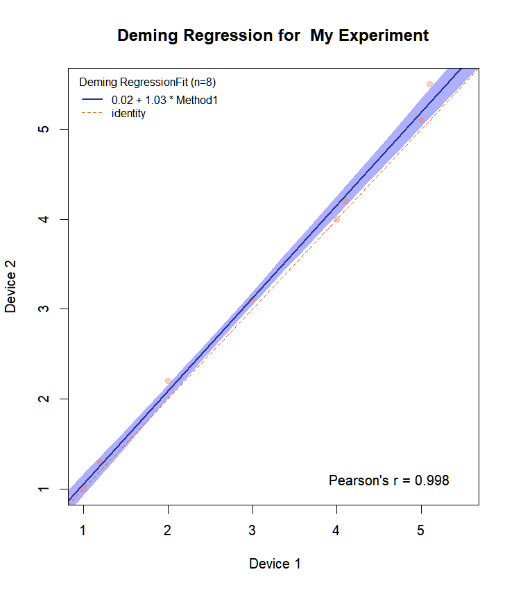
我们注意到,对于这个玩具数据来说,上述一致性几乎是完美的。斜率等于 1,置信区间为 0.97-1.09。函数 MCResult.plot 默认也用所选颜色绘制置信区间。它还会在图中标出方程。
如果想把斜率和截距的 CI 也放在图上,下面是对 MCResult.plot() 函数的修改:
MCResult.plot2 0 & alpha = length(names(digits)))
  如果 (is.null(digits$coef)) {
    digits$coef <- 2
  }
  如果 (is.null(digits$cor)) {
    digits$cor <- 3
  }
  cor.method <- match.arg(cor.method)
  stopifnot(is.element(cor.method, c("pearson", "kendall"、
                                     "spearman"))
  legend.place  1)
    stopifnot(length(points.col) == nrow(x@data))
  if (length(points.pch) > 1)
    stopifnot(length(points.pch) == nrow(x@data))
  if (x@regmeth == "LinReg")
    titname <- "线性回归"
  else if (x@regmeth == "WLinReg")
    titname <- "加权线性回归"
  else if (x@regmeth == "TS")
    titname <- "Theil-Sen 回归"
  else if (x@regmeth == "PBequi")
    titname <- "等变传递-Bablok 回归"
  else if (x@regmeth == "Deming")
    titname <- "戴明回归"
  else if (x@regmeth == "WDeming")
    titname <- "加权戴明回归"
  else titname <- "传递巴布洛克回归"
  niceblue <- rgb(37/255, 52/255, 148/255)
  niceor <- rgb(230/255, 85/255, 13/255)
  niceblue.bounds <- rgb(236/255, 231/255, 242/255)
  if (is.null(reg.col))
    reg.col <- niceblue
  if (is.null(identity.col))
    identity.col <- niceor
  if (is.null(ci.area.col))
    ci.area.col <- niceblue.bounds
  if (is.null(ci.border.col))
    ci.border.col  1)
  if (is.null(xlim))
    rx <- range(x@data[, "x"], na.rm = TRUE)
  else rx <- xlim
  tmp.range <- range(as.vector(x@data[, c("x", "y")]), na.rm = TRUE)
  if (equal.axis == TRUE) {
    if (is.null(ylim)) {
      yrange <- tmp.range
    }
    否则 {
      yrange <- ylim
    }
  }
  else {
    if (is.null(ylim)) {
      yrange <- range(as.vector(x@data[, "y"]), na.rm = TRUE)
    }
    else {
      yrange <- ylim
    }
  }
  if (!is.null(xlim) && !is.null(ylim) && equal.axis) {
    xlim <- c(min(c(xlim[1], ylim[1])), max(c(xlim[2], ylim[2])))
  }
  if (is.null(xaxp)){
    if (!is.null(xlim)) {
      axis_ticks <- axisTicks(c(xlim[1] - 0.05 * xlim[2]、
                                ceiling((xlim[2] + 0.05 * xlim[2]) * 10^digits$coef)/10^digits$coef)、
                              log = F, nint = 7)
      xaxp <- c(axis_ticks[1], tail(axis_ticks, n = 1)、
                length(axis_ticks) - 1)
      xlim <- c(axis_ticks[1], tail(axis_ticks, n = 1))
    }
  }
  否则 {
    if (!is.null(xlim)) {
      if ((xlim[1] == rx[1] && xlim[2] == rx[2]) | (tmp.range[1] ==
                                                    xlim[1] && tmp.range[2] == xlim[2])){
        xlim <- c(xaxp[1], xaxp[2])
      }
    }
    否则 {
      warning("xaxp 绝不应在没有 xlim 的情况下设置")
      xaxp <- NULL
    }
  }
  if (is.null(yaxp)){
    if (!is.null(ylim) && !equal.axis) {
      yaxp <- axis_ticks <- axisTicks(c(ylim[1] - 0.05 *.
                                          ylim[2], ceiling((ylim[2] + 0.05 * ylim[2]) *
                                                             10^digits$coef)/10^digits$coef), log = F, nint = 10)
      yaxp = c(axis_ticks[1], tail(axis_ticks, n = 1)、
               length(axis_ticks) - 1)
      ylim <- c(axis_ticks[1], tail(axis_ticks, n = 1))
    }
    否则 {
      if (equal.axis) {
        if (!is.null(xlim)) {
          yaxp <- xaxp
          ylim <- xlim
        }
      }
    }
  }
  else {
    if (!is.null(ylim)) {
      如果 ((ylim[1] == yrange[1] && ylim[2] == yrange[2]) |
          (tmp.range[1] == ylim[1] && tmp.range[2] == ylim[2])){
        ylim <- c(yaxp[1], yaxp[2])
      }
    }
    否则 {
      warning("yaxp 不应在没有 ylim 的情况下设置")
      yaxp <- NULL
    }
  }
  if (equal.axis) {
    if (is.null(ylim)) {
      yaxp <- xaxp
      ylim <- xlim
    }
    if (is.null(xlim)) {
      xaxp <- yaxp
      xlim <- ylim
    }
  }
  if (!is.null(xlim)) {
    if (xlim[1] < tmp.range[1]) {
      tmp.range[1]  tmp.range[2]) {
      tmp.range[2] <- xlim[2]
    }
  }
  if (!is.null(ylim)) {
    if (ylim[1] < yrange[1]) {
      yrange[1]  yrange[2]) {
      yrange[2]  yrange[2])
    }
  }
  xd <- seq(rx[1], rx[2], length.out = xn)
  xd <- union(xd, rx)
  delta <- abs(rx[1] - rx[2])/xn
  xd <- xd[order(xd)]
  xd.add <- c(xd[1] - delta * 1:10, xd, xd[length(xd)] + delta * 1:10)
                1:10)
  if (is.null(xlim))
    xlim <- rx
  if (ci.area == TRUE | ci.border == TRUE) {
    bounds <- calcResponse(x, alpha = alpha, x.levels = xd)
    bounds.add <- calcResponse(x, alpha = alpha, x.levels = xd.add)
    if (equal.axis == TRUE) {
      xd <- seq(tmp.range[1], tmp.range[2], length.out = xn)
      xd <- union(xd, tmp.range)
      delta <- abs(rx[1] - rx[2])/xn
      xd <- xd[order(xd)]
      xd.add <- c(xd[1] - delta * 1:10, xd, xd[length(xd)] +
                    delta * 1:10)
      bounds <- calcResponse(x, alpha = alpha, x.levels = xd)
      bounds.add <- calcResponse(x, alpha = alpha, x.levels = xd.add)
      yrange <- range(c(as.vector(x@data[, c("x", "y")])、
                        as.vector(bounds[, c("X", "Y", "Y.LCI", "Y.UCI")])、
                      na.rm = TRUE)
    }
    else {
      yrange <- range(c(as.vector(x@data[, "y"]), as.vector(bounds[、
                                                                   c("Y", "Y.LCI", "Y.UCI")]), na.rm = TRUE)
    }
  }
  否则 {
    if (equal.axis == TRUE) {
      yrange <- tmp.range
    }
    else {
      yrange <- range(as.vector(x@data[, "y"]), na.rm = TRUE)
    }
  }
  if (equal.axis) {
    if (is.null(ylim)) {
      xlim <- ylim <- tmp.range
    }
    else {
      xlim <- ylim
    }
  }
  else {
    if (is.null(xlim))
      xlim <- rx
    if (is.null(ylim))
      ylim <- yrange
  }
  if (is.null(main))
    main <- paste(titname, "Fit")
  if (!add) {
    plot(0, 0, cex = 0, ylim = ylim, xlim = xlim, xlab = x.lab、
         ylab = y.lab, main = main, sub = "", xaxp = xaxp、
         yaxp = yaxp, bty = "n", ...)
  }
  else {
    sub <- ""
    add.legend <- FALSE
    add.grid <- FALSE
  }
  if (add.legend == TRUE) {
    if (identity == TRUE & reg == TRUE) {
      text2 <- "身份"
      text1 <- paste(formatC(round(x@para["Intercept"、
                                          "EST"], digits = digits$coef), digits = digits$coef、
                             format = "f"),"(",formatC(round(x@para["Intercept"、
                                                                    "LCI"], digits = digits$coef), digits = digits$coef、
                                                       format = "f"),";",formatC(round(x@para["Intercept"、
                                                                                          "UCI"], digits = digits$coef), digits = digits$coef、
                                                                             format = "f"),")"," + ", formatC(round(x@para["Slope"、
                                                                        "EST"], digits = digits$coef), digits = digits$coef、
                                                           format = "f"),"(",formatC(round(x@para["Slope"、
                                                                                                  "LCI"], digits = digits$coef), digits = digits$coef、
                                                                                     format = "f"),";",formatC(round(x@para["Slope"、
                                                                                                                        "UCI"], digits = digits$coef), digits = digits$coef、
                                                                                                           format = "f"),")"," * ", x@mnames[1], sep = "")
      legend(legend.place, lwd = c(reg.lwd, identity.lwd)、
             lty = c(reg.lty, identity.lty), col = c(reg.col、
                                                     identity.col), title = paste(titname, "Fit (n="、
                                                                                  dim(x@data)[1], ")", sep = ""), legend = c(text1、
                                                                                                                             text2), box.lty = "blank", cex = 0.8, bg = "white"、
             inset = c(0.01, 0.01))
    }
    if (identity == TRUE & reg == FALSE) {
      text2 <- "身份"
      legend(legend.place, lwd = identity.lwd, lty = identity.lty、
             col = identity.col, title = paste(titname, "Fit (n="、
                                               dim(x@data)[1], ")", sep = ""), legend = text2、
             box.lty = "blank", cex = 0.8, bg = "white", inset = c(0.01、
                                                                   0.01))
    }
    if (identity == FALSE & reg == TRUE) {
      text1 <- paste(formatC(round(x@para["Intercept"、
                                          "EST"], digits = digits$coef), digits = digits$coef、
                             format = "f"), "+", formatC(round(x@para["Slope"、
                                                                      "EST"],digits = digits$coef),digits = digits$coef、
                                                         format = "f"), "*", x@mnames[1], sep = "")
      legend(legend.place, lwd = c(2), col = c(reg.col)、
             title = paste(titname, "Fit (n=", dim(x@data)[1]、
                           ")", sep = ""), legend = c(text1), box.lty = "blank"、
             cex = 0.8, bg = "white", inset = c(0.01, 0.01))
    }
  }
  if (ci.area == TRUE | ci.border == TRUE) {
    if (ci.area == TRUE) {
      xxx <- c(xd.add, xd.add[order(xd.add, decreasing = TRUE)])
      yy1 <- c(as.vector(bounds.add[, "Y.LCI"]))
      yy2 <- c(as.vector(bounds.add[, "Y.UCI"]))
      yyy <- c(yy1, yy2[order(xd.add, decreasing = TRUE)])
      polygon(xxx, yyy, col = ci.area.col, border = "white"、
              lty = 0)
    }
    if (add.grid)
      网格()
    if (ci.border == TRUE) {
      points(xd.add, bounds.add[, "Y.LCI"], lty = ci.border.lty、
             lwd = ci.border.lwd,type = "l",col = ci.border.col)
      points(xd.add, bounds.add[, "Y.UCI"], lty = ci.border.lty、
             lwd = ci.border.lwd,type = "l",col = ci.border.col)
    }
    if (is.null(sub)) {
      if (x@cimeth %in% c("bootstrap", "nestedbootstrap"))
        subtext <- paste("The ", 1 - x@alpha, "-confidence bounds are calculated with the "、
                         x@cimeth, "(", x@bootcimeth, ") 方法计算。", sep = "")
      else if ((x@regmeth =="PaBa") & (x@cimeth =="analytical"))
        subtext <- ""
      else subtext <- paste("The ", 1 - x@alpha, "-confidence bounds are calculated with the "、
                            x@cimeth, " 方法计算。", sep = "")
    }
    else subtext <- sub
  }
  else {
    if (add.grid)
      grid()
    subtext <- ifelse(is.null(sub), "", sub)
  }
  if (add.cor == TRUE) {
    cor.coef <- paste(formatC(round(cor(x@data[, "x"], x@data[、
                                                              "y"], use = "pairwise.complete.obs", method = cor.method)、
                                    digits = digits$cor), digits = digits$cor, format = "f"))
    if (cor.method == "pearson")
      cortext <- paste("Pearson's r = ", cor.coef, sep = "")
    if (cor.method == "kendall")
      cortext <- bquote(paste("Kendall's ", tau, " = "、
                              .(cor.coef), sep = ""))
    if (cor.method == "spearman")
      cortext <- bquote(paste("Spearman's ", rho, " = "、
                              .(cor.coef), sep = ""))
    mtext(side = 1, line = -2, cortext, adj = 0.9, font = 1)
  }
  if (draw.points == TRUE) {
    points(x@data[, 2:3], col = points.col, pch = points.pch、
           cex = points.cex, ...)
  }
  title(sub = subtext)
  if (reg == TRUE) {
    b0 <- x@para["Intercept", "EST"]
    b1 <- x@para["斜率", "EST"]
    abline(b0, b1, lty = reg.lty, lwd = reg.lwd, col = reg.col)
  }
  if (identity == TRUE) {
    abline(0, 1, lty = identity.lty, lwd = identity.lwd、
           col = identity.col)
  }
  box()
}
如果我们现在改变函数
Draw.Deming.Plot<-function(resp1,resp2,name1){
  #mcreg 不接受 NA
  df<-as.data.frame(cbind(resp1,resp2))
  df2<-df[complete.cases(df),]
  dem.reg <- mcreg(df2$resp1,df2$resp2, error.ratio = 1, method.reg = "Deming")
  MCResult.plot2(dem.reg, equal.axis = TRUE, x.lab = " 设备 1", y.lab = "设备 2", points.col = "#FF7F5060", points.pch = 19, ci.area = TRUE, ci.area.col = "#0000FF50", main = paste("Deming Regression for ",name1), sub = "", add.grid = FALSE, points.cex = 1)
  return(list(intercept=c(dem.reg@para[1,c(1,3,4)]),slope=c(dem.reg@para[2,c(1,3,4)]))
}
我们呼叫
Draw.Deming.Plot(resp1,resp2, "My Experiment")然后我们得到
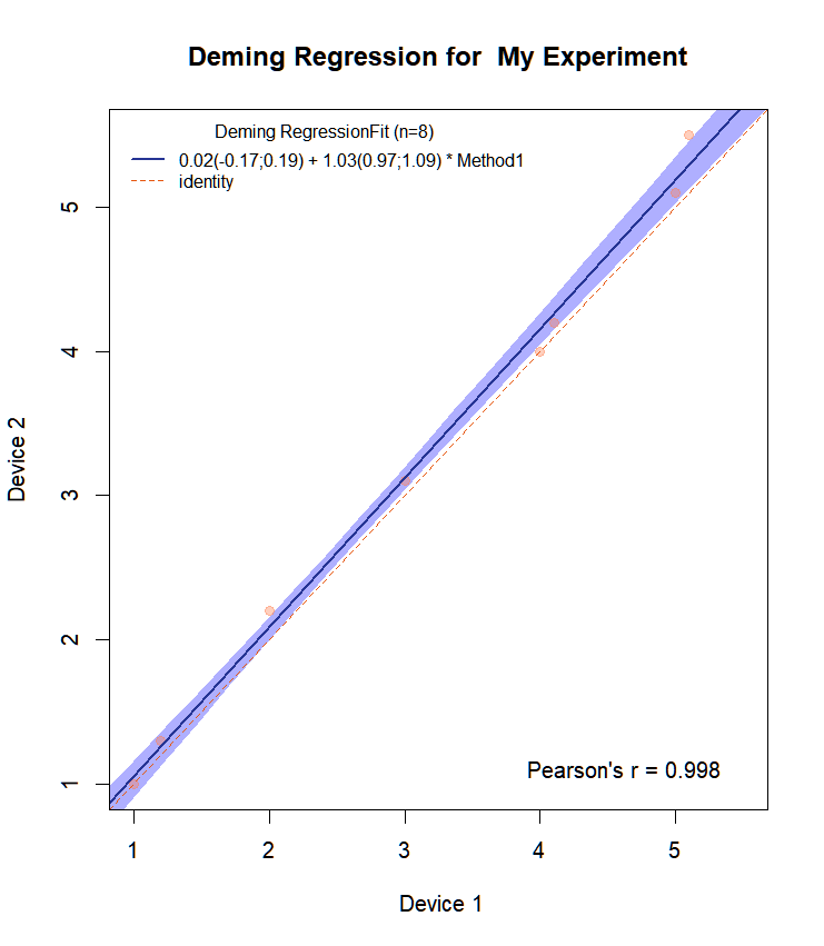
现在,曲线图上的斜率和截距都是 CI。
玩得开心!