

Wir alle kennen die gängigen linearen OLS-Regressionsmodelle. Bei dieser Art von Modellen gehen wir davon aus, dass Y linear von einem, nehmen wir an, kontinuierlichen Prädiktor X plus abhängt, und wir berücksichtigen den Messfehler für Y als:
Y_i=A+B*X_i,
i ist der Index der i-ten Beobachtung in X und Y.
Da es nur einen Prädiktor gibt, kann der lineare Korrelationskoeffizient R anhand dieses Regressionsmodells wie folgt geschätzt werden:
r=R=sqrt(R^2).
Beachten Sie auch, dass die Prüfung von H0:r=0 gleichbedeutend ist mit der Prüfung von H0:B=0.
X kann z. B. die Zeit sein, die der i-te Student für das Lernen aufgewendet hat, und X sein Ergebnis in der Prüfung.
Im Idealfall ist Y umso höher, je länger X ist, so dass der Koeffizient B positiv sein sollte.
Die Anpassung dieses Modells in R erfolgt über eine Funktion:
lm(Y~X, data=my.data)Was aber, wenn wir zum Beispiel zwei Geräte Dev1 und Dev2 vergleichen wollen. Wir messen das Gleiche auf Dev1 und Dev2. Als Ergebnis erhalten wir den Vektor der Messwerte für Dev1 (X1) und Dev2 (X2). Die Bewertung der Übereinstimmung zwischen diesen beiden Maschinen erfolgt über eine so genannte Deming-Regression. Diese Regression ist der OLS-Regression ähnlich, geht aber davon aus, dass sowohl Y als auch X mit Fehlern gemessen werden.
Daher gilt für das erste Gerät Dev1:
X1_i=A1+B1*TrueX1_i+E2_i
Und für das zweite Gerät DEV2:
X2_i=A2+B2*TrueX2_i+E2_i.
In den obigen Gleichungen sind E1 und E2 die Messfehler.
Wir nehmen an, dass diese Fehlervektoren normalverteilt sind mit N(0,sigma1^2) und N(0,sigma2^2). Außerdem definieren wir lambda=sigma1^2/sigma2^2.
Das Lambda ist das Verhältnis der Varianz der beiden Messfehler. Normalerweise nehmen wir Lambda=1 an, damit keine der Maschinen im Vorteil ist. Die Anpassung der Deming-Regression in R erfolgt über das Paket mcr.
Im Folgenden habe ich eine Funktion geschrieben, die das Ergebnis der Deming-Regression zeichnet, die mit der Funktion mcreg angepasst wird.
Sie liefert auch die Steigung und den Achsenabschnitt des Modells.
Draw.Deming.Plot<-function(resp1,resp2,name1){
  #mcreg akzeptiert keine NAs
  df<-as.data.frame(cbind(resp1,resp2))
  df2<-df[complete.cases(df),]
  dem.reg <- mcreg(df2$resp1,df2$resp2, error.ratio = 1, method.reg = "Deming")
  MCResult.plot(dem.reg, equal.axis = TRUE, x.lab = "Gerät 1", y.lab = "Gerät 2", points.col = "#FF7F5060", points.pch = 19, ci.area = TRUE, ci.area.col = "#0000FF50", main = paste("Deming Regression für ",name1), sub = "", add.grid = FALSE, points.cex = 1)
  return(list(intercept=c(dem.reg@para[1,c(1,3,4)]),slope=c(dem.reg@para[2,c(1,3,4)])))
}
Sehen wir uns das Diagramm an, das für die Beispieldaten resp1 und resp2 erstellt wird.
resp1<-c(1,1.2,2,3,4,4.1,5,5.1)
resp2<-c(1,1.3,2.2,3.1,4,4.2,5.1,5.5)
Draw.Deming.Plot(resp1,resp2, "Mein Experiment")
Wir bekommen:
1TP3Abschnitt
        EST LCI UCI
 0.01532475 -0.18087790 0.19446184

$Steigung
      EST LCI UCI
1.0345434 0.9672911 1.0910989
Und die Handlung:
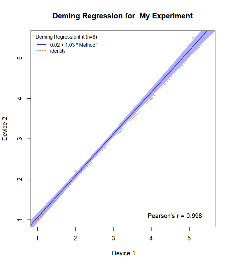
Wir stellen fest, dass die obige Übereinstimmung für diese Spielzeugdaten nahezu perfekt ist. Die Steigung ist gleich 1 mit CI: 0,97-1,09. Die Funktion MCResult.plot stellt standardmäßig auch die Vertrauensbereiche in der gewählten Farbe dar. Sie fügt auch die Gleichung in das Diagramm ein.
Wenn man auch die KI für die Steigung und den Achsenabschnitt auf dem Diagramm darstellen möchte, ist hier die Modifikation der Funktion MCResult.plot():
MCResult.plot2 0 & alpha = Länge(Namen(Ziffern)))
  if (is.null(Ziffern$coef)) {
    Ziffern$coef <- 2
  }
  if (is.null(Ziffern$cor)) {
    Ziffern$cor <- 3
  }
  cor.method <- match.arg(cor.method)
  stopifnot(is.element(cor.method, c("pearson", "kendall",
                                     "spearman")))
  legend.place  1)
    stopifnot(length(points.col) == nrow(x@data))
  if (length(points.pch) > 1)
    stopifnot(length(points.pch) == nrow(x@data))
  if (x@regmeth == "LinReg")
    titname <- "Lineare Regression"
  else if (x@regmeth == "WLinReg")
    Titelname <- "Gewichtete lineare Regression"
  sonst wenn (x@regmeth == "TS")
    Titelname <- "Theil-Sen Regression"
  sonst if (x@regmeth == "PBequi")
    Titelname <- "Äquivariante Passing-Bablok-Regression"
  sonst if (x@regmeth == "Deming")
    Titelname <- "Deming-Regression"
  sonst if (x@regmeth == "WDeming")
    titname <- "Gewichtete Deming-Regression"
  sonst titname <- "Passing Bablok Regression"
  niceblue <- rgb(37/255, 52/255, 148/255)
  niceor <- rgb(230/255, 85/255, 13/255)
  niceblue.bounds <- rgb(236/255, 231/255, 242/255)
  if (is.null(reg.col))
    reg.col <- niceblue
  if (is.null(identity.col))
    identität.spalte <- niceor
  if (is.null(ci.area.col))
    ci.area.col <- niceblue.bounds
  if (is.null(ci.border.col))
    ci.border.col  1)
  if (is.null(xlim))
    rx <- Bereich(x@Daten[, "x"], na.rm = TRUE)
  sonst rx <- xlim
  tmp.range <- range(as.vector(x@data[, c("x", "y")]), na.rm = TRUE)
  if (equal.axis == TRUE) {
    if (is.null(ylim)) {
      ybereich <- tmp.bereich
    }
    sonst {
      ybereich <- ylim
    }
  }
  else {
    if (is.null(ylim)) {
      yrange <- range(as.vector(x@data[, "y"]), na.rm = TRUE)
    }
    else {
      ybereich <- ylim
    }
  }
  if (!is.null(xlim) && !is.null(ylim) && equal.axis) {
    xlim <- c(min(c(xlim[1], ylim[1])), max(c(xlim[2], ylim[2])))
  }
  if (is.null(xaxp)) {
    if (!is.null(xlim)) {
      axis_ticks <- axisTicks(c(xlim[1] - 0.05 * xlim[2],
                                ceiling((xlim[2] + 0.05 * xlim[2]) * 10^digits$coef)/10^digits$coef),
                              log = F, nint = 7)
      xaxp <- c(axis_ticks[1], tail(axis_ticks, n = 1),
                length(axis_ticks) - 1)
      xlim <- c(axis_ticks[1], tail(axis_ticks, n = 1))
    }
  }
  else {
    if (!is.null(xlim)) {
      if ((xlim[1] == rx[1] && xlim[2] == rx[2]) | (tmp.range[1] ==
                                                    xlim[1] && tmp.range[2] == xlim[2])) {
        xlim <- c(xaxp[1], xaxp[2])
      }
    }
    else {
      warning("xaxp sollte nie ohne xlim gesetzt werden")
      xaxp <- NULL
    }
  }
  if (is.null(yaxp)) {
    if (!is.null(ylim) && !equal.axis) {
      yaxp <- axis_ticks <- axisTicks(c(ylim[1] - 0.05 *
                                          ylim[2], ceiling((ylim[2] + 0.05 * ylim[2]) *
                                                             10^digits$coef)/10^digits$coef), log = F, nint = 10)
      yaxp = c(axis_ticks[1], tail(axis_ticks, n = 1),
               length(axis_ticks) - 1)
      ylim <- c(axis_ticks[1], tail(axis_ticks, n = 1))
    }
    else {
      if (equal.axis) {
        if (!is.null(xlim)) {
          yaxp <- xaxp
          ylim <- xlim
        }
      }
    }
  }
  else {
    if (!is.null(ylim)) {
      if ((ylim[1] == yrange[1] && ylim[2] == yrange[2]) |
          (tmp.range[1] == ylim[1] && tmp.range[2] == ylim[2])) {
        ylim <- c(yaxp[1], yaxp[2])
      }
    }
    else {
      warning("yaxp sollte nie ohne ylim gesetzt werden")
      yaxp <- NULL
    }
  }
  if (equal.axis) {
    if (is.null(ylim)) {
      yaxp <- xaxp
      ylim <- xlim
    }
    if (is.null(xlim)) {
      xaxp <- yaxp
      xlim <- ylim
    }
  }
  if (!is.null(xlim)) {
    if (xlim[1] < tmp.range[1]) {
      tmp.bereich[1]  tmp.bereich[2]) {
      tmp.bereich[2] <- xlim[2]
    }
  }
  if (!is.null(ylim)) {
    if (ylim[1] < yrange[1]) {
      yrange[1]  yrange[2]) {
      yrange[2] <- ylim[2]
    }
  }
  xd <- seq(rx[1], rx[2], length.out = xn)
  xd <- union(xd, rx)
  delta <- abs(rx[1] - rx[2])/xn
  xd <- xd[order(xd)]
  xd.add <- c(xd[1] - delta * 1:10, xd, xd[length(xd)] + delta *
                1:10)
  if (is.null(xlim))
    xlim <- rx
  if (ci.area == TRUE | ci.border == TRUE) {
    bounds <- calcResponse(x, alpha = alpha, x.levels = xd)
    bounds.add <- calcResponse(x, alpha = alpha, x.levels = xd.add)
    if (equal.axis == TRUE) {
      xd <- seq(tmp.range[1], tmp.range[2], length.out = xn)
      xd <- union(xd, tmp.bereich)
      delta <- abs(rx[1] - rx[2])/xn
      xd <- xd[order(xd)]
      xd.add <- c(xd[1] - delta * 1:10, xd, xd[length(xd)] +
                    delta * 1:10)
      bounds <- calcResponse(x, alpha = alpha, x.levels = xd)
      bounds.add <- calcResponse(x, alpha = alpha, x.levels = xd.add)
      yrange <- range(c(as.vector(x@data[, c("x", "y")]),
                        as.vector(bounds[, c("X", "Y", "Y.LCI", "Y.UCI")])),
                      na.rm = TRUE)
    }
    else {
      yrange <- range(c(as.vector(x@data[, "y"]), as.vector(bounds[,
                                                                   c("Y", "Y.LCI", "Y.UCI")])), na.rm = TRUE)
    }
  }
  sonst {
    if (equal.axis == TRUE) {
      ybereich <- tmp.bereich
    }
    sonst {
      yrange <- range(as.vector(x@data[, "y"]), na.rm = TRUE)
    }
  }
  if (equal.axis) {
    if (is.null(ylim)) {
      xlim <- ylim <- tmp.range
    }
    else {
      xlim <- ylim
    }
  }
  else {
    if (is.null(xlim))
      xlim <- rx
    if (is.null(ylim))
      ylim <- yrange
  }
  if (is.null(main))
    main <- paste(titname, "Fit")
  if (!add) {
    plot(0, 0, cex = 0, ylim = ylim, xlim = xlim, xlab = x.lab,
         ylab = y.lab, main = main, sub = "", xaxp = xaxp,
         yaxp = yaxp, bty = "n", ...)
  }
  else {
    sub <- ""
    add.legend <- FALSE
    add.grid <- FALSE
  }
  if (add.legend == TRUE) {
    if (identität == TRUE & reg == TRUE) {
      text2 <- "identität"
      text1 <- paste(formatC(round(x@para["Intercept",
                                          "EST"], digits = digits$coef), digits = digits$coef,
                             format = "f"),"(",formatC(round(x@para["Intercept",
                                                                    "LCI"], Ziffern = digits$coef), Ziffern = digits$coef,
                                                       format = "f"),";",formatC(round(x@para["Achsenabschnitt",
                                                                                          "UCI"], Ziffern = digits$coef), Ziffern = digits$coef,
                                                                             format = "f"),")"," + ", formatC(round(x@para["Steigung",
                                                                        "EST"], Ziffern = digits$coef), Ziffern = digits$coef,
                                                           format = "f"),"(",formatC(round(x@para["Steilheit",
                                                                                                  "LCI"], Ziffern = digits$coef), Ziffern = digits$coef,
                                                                                     format = "f"),";",formatC(round(x@para["Steilheit",
                                                                                                                        "UCI"], Ziffern = digits$coef), Ziffern = digits$coef,
                                                                                                           format = "f"),")" ," * ", x@mnames[1], sep = "")
      legend(legend.place, lwd = c(reg.lwd, identity.lwd),
             lty = c(reg.lty, identity.lty), col = c(reg.col,
                                                     identity.col), title = paste(titname, "Fit (n=",
                                                                                  dim(x@data)[1], ")", sep = ""), legend = c(text1,
                                                                                                                             text2), box.lty = "leer", cex = 0.8, bg = "weiß",
             inset = c(0.01, 0.01))
    }
    if (identity == TRUE & reg == FALSE) {
      text2 <- "identität"
      legend(legend.place, lwd = identity.lwd, lty = identity.lty,
             col = identity.col, title = paste(titname, "Fit (n=",
                                               dim(x@data)[1], ")", sep = ""), legend = text2,
             box.lty = "blank", cex = 0.8, bg = "white", inset = c(0.01,
                                                                   0.01))
    }
    if (identity == FALSE & reg == TRUE) {
      text1 <- paste(formatC(round(x@para["Intercept",
                                          "EST"], digits = digits$coef), digits = digits$coef,
                             format = "f"), "+", formatC(round(x@para["Steigung",
                                                                      "EST"], Ziffern = digits$coef), digits = digits$coef,
                                                         format = "f"), "*", x@mnames[1], sep = "")
      legend(legend.place, lwd = c(2), col = c(reg.col),
             title = paste(titname, "Fit (n=", dim(x@data)[1],
                           ")", sep = ""), legend = c(text1), box.lty = "blank",
             cex = 0.8, bg = "weiß", inset = c(0.01, 0.01))
    }
  }
  if (ci.area == TRUE | ci.border == TRUE) {
    if (ci.area == TRUE) {
      xxx <- c(xd.add, xd.add[order(xd.add, decreasing = TRUE)])
      yy1 <- c(as.vector(bounds.add[, "Y.LCI"]))
      yy2 <- c(as.vector(bounds.add[, "Y.UCI"]))
      yyy <- c(yy1, yy2[order(xd.add, decreasing = TRUE)])
      polygon(xxx, yyy, col = ci.area.col, border = "white",
              lty = 0)
    }
    if (add.grid)
      grid()
    if (ci.border == TRUE) {
      points(xd.add, bounds.add[, "Y.LCI"], lty = ci.border.lty,
             lwd = ci.border.lwd, type = "l", col = ci.border.col)
      points(xd.add, bounds.add[, "Y.UCI"], lty = ci.border.lty,
             lwd = ci.border.lwd, type = "l", col = ci.border.col)
    }
    if (is.null(sub)) {
      if (x@cimeth %in% c("bootstrap", "nestedbootstrap"))
        subtext <- paste("Die ", 1 - x@alpha, "-Konfidenzintervalle werden mit dem ",
                         x@cimeth, "(", x@bootcimeth, ") Methode berechnet.", sep = "")
      else if ((x@regmeth == "PaBa") & (x@cimeth == "analytisch"))
        subtext <- ""
      else subtext <- paste("Die ", 1 - x@alpha, "-Vertrauensbereiche werden mit der ",
                            x@cimeth, " Methode.", sep = "")
    }
    sonst subtext <- sub
  }
  else {
    if (add.grid)
      grid()
    subtext <- ifelse(is.null(sub), "", sub)
  }
  if (add.cor == TRUE) {
    cor.coef <- paste(formatC(round(cor(x@data[, "x"], x@data[,
                                                              "y"], use = "pairwise.complete.obs", method = cor.method),
                                    Ziffern = Ziffern$cor), Ziffern = Ziffern$cor, Format = "f"))
    if (cor.method == "pearson")
      cortext <- paste("Pearson's r = ", cor.coef, sep = "")
    if (cor.method == "kendall")
      cortext <- bquote(paste("Kendall's ", tau, " = ",
                              .(cor.coef), sep = ""))
    if (cor.method == "spearman")
      cortext <- bquote(paste("Spearman's ", rho, " = ",
                              .(cor.coef), sep = ""))
    mtext(side = 1, line = -2, cortext, adj = 0.9, font = 1)
  }
  if (draw.points == TRUE) {
    points(x@data[, 2:3], col = points.col, pch = points.pch,
           cex = points.cex, ...)
  }
  title(sub = subtext)
  if (reg == TRUE) {
    b0 <- x@para["Achsenabschnitt", "EST"]
    b1 <- x@para["Steigung", "EST"]
    abline(b0, b1, lty = reg.lty, lwd = reg.lwd, col = reg.col)
  }
  if (identity == TRUE) {
    abline(0, 1, lty = identity.lty, lwd = identity.lwd,
           col = identity.col)
  }
  box()
}
Wenn wir jetzt die Funktion ändern:
Draw.Deming.Plot<-function(resp1,resp2,name1){
  #mcreg akzeptiert keine NAs
  df<-as.data.frame(cbind(resp1,resp2))
  df2<-df[complete.cases(df),]
  dem.reg <- mcreg(df2$resp1,df2$resp2, error.ratio = 1, method.reg = "Deming")
  MCResult.plot2(dem.reg, equal.axis = TRUE, x.lab = "Gerät 1", y.lab = "Gerät 2", points.col = "#FF7F5060", points.pch = 19, ci.area = TRUE, ci.area.col = "#0000FF50", main = paste("Deming Regression für ",name1), sub = "", add.grid = FALSE, points.cex = 1)
  return(list(intercept=c(dem.reg@para[1,c(1,3,4)]),slope=c(dem.reg@para[2,c(1,3,4)])))
}
Und wir rufen an:
Draw.Deming.Plot(resp1,resp2, "Mein Experiment")Dann bekommen wir:
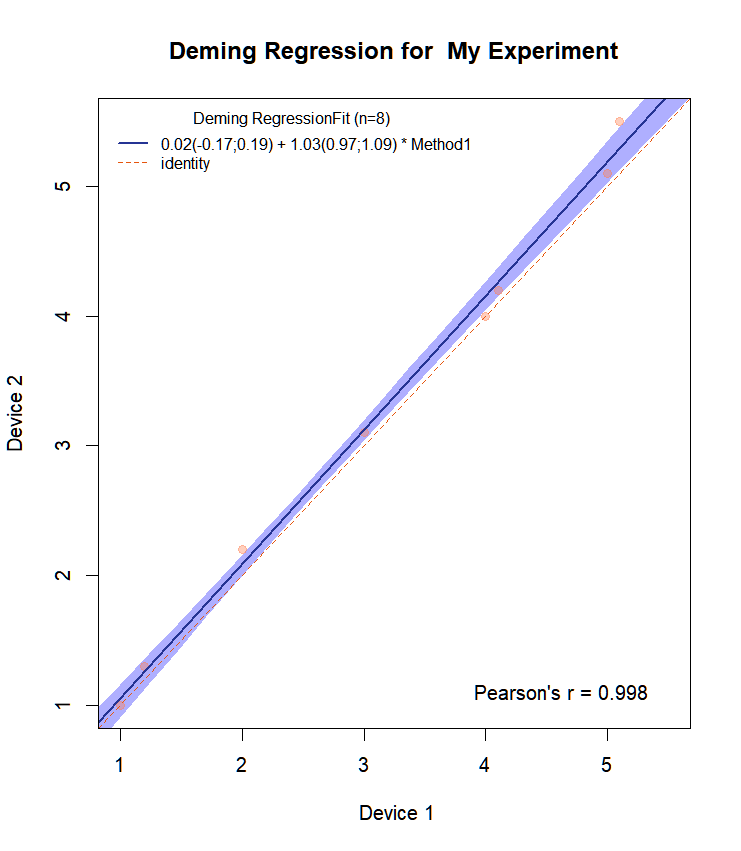
Es hat jetzt alle CI für die Steigung und den Achsenabschnitt auf dem Diagramm.
Viel Spaß!